Staying On Top Of Your Business Numbers With Power BI Automatic Reports

With Power BI, I easily monitor my website performance and see the important figures from any device I am on. Also, I am able to monitor my business finance -- track sales, invoices, expenses and instantly generate financial reports. And same for my email marketing campaigns. All in one central place. And you know the best part? The reports are automatically generated for me and updated daily. No need to have a staff make me reports or depend on my now less reliable memory to remind me to generate the report.

And what if I tell you that all these are free and can be easily set-up by you. All you have to do is sign up for Power BI.

Sign up is very easy. Then log in afterwards. You will be directed to a page similar to the one below.

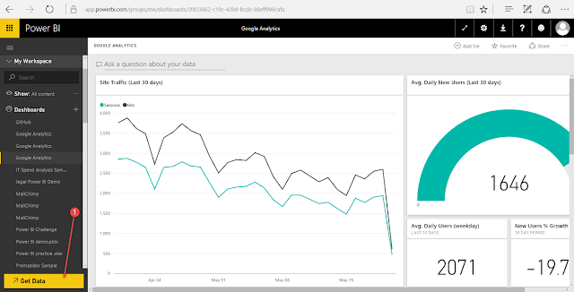
And immediately redirected to the Power BI dashboard. In your case, you will see Microsoft sample reports. I have connected mine to my Google Analytics to monitor my website performance, Mailchimp to check the performance of my email marketing and QuickBooks to see my business performance.

Google Analytics Automated Report

Mailchimp Automated Report

QuickBooks Automated Report

So how did I initiate the report generation? Very easy. I simply connect Power BI to my Google Analytics account, Mailchimp account and QuickBooks account. And that's all. Power BI will generate a comprehensive report that shows you the important numbers all by itself. And if you want, you can customize the reports or add more analysis.

Just click on "Get Data" at the lower left corner to get started.

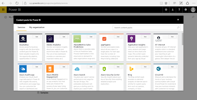
Choose "Services".

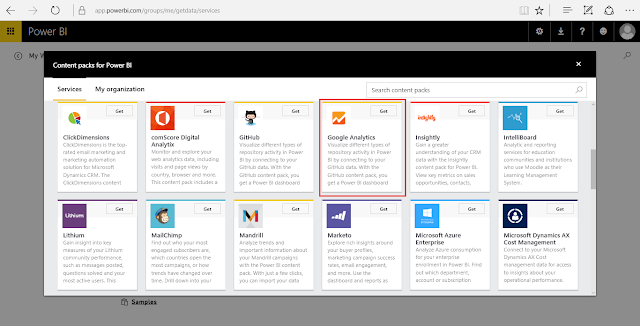
A list of all the services you can connect to will come up. Click "Get" on the ones you want the automatic report generated for.

Notice the detailed report of my business finances from QuickBooks

And that is all.

And if you are a smartphone person, like most of us, you should install the Power BI app from your phone app store (available for Windows Phone, Android and iPhone). So you can always view your reports on your phone. And it automatically updates everyday. No need for you to recreate the report or refresh or update. It does that daily for you without your intervention. That way you always see the most recent report.

The Amazing Tool Called Data Table In Excel

In Excel, there is an amazing tool called Data Table. It lets you sort of simulate a lot of predefined conditions.

For illustration, I'll create an example we can all relate with. It's the revenue projections of a small vibrant company.

There is a formula in the Revenue field that depends on the Product Price and Marketing Cost.

The next thing, we will do is help the management simulate what the Revenue will be for different combinations of Product Price and Marketing Cost.

This is the sort of task Data Table is great at.

All we have to do is link the cell at the junction of the simulated Product Price and simulated Marketing Cost to the calculated Revenue cell. See the screenshot below for what I mean.

Now we are ready to use Data Table.

Select the entire simulation table.

Then go to Data menu, What-If Analysis and Data Table.

In the small dialog box that comes up, set the Row Input Cell to the Marketing Cost value in the analysis table. And set the Column Input Cell to the Product Price in the analysis table.

And you get what the Revenue will be for the different combinations of Product Price and Marketing Cost.

It's now left for the management of Vibrant Nigeria Limited to choose which combination of Product Price and Marketing Cost will get them the best Profit after factoring the Cost of Sales.

You can register for our upcoming intensive Business Data Analysis and Microsoft Excel training here.

How To Pick Items From A List Using CHOOSE

CHOOSE is one of the formulas dedicated to making your analysis life easier. You can easily do dynamic reports just by using CHOOSE.

I have an illustration we can all easily understand. It is Sam's todo list for the day. A list of 10 tasks he has arranged in the order he intends to carry them out today.

In reality, you would want to use CHOOSE for something more complex. But the concept is the same and once you grasp how to use it here, you can use it anywhere -- even for a list of 100,000 entries in a different Excel file.

Back to our illustration.

Sam wants a simple way to see the progress he is making. He wants to type in a task number and see what it is about and if he has done it. And this where CHOOSE comes in very handy.

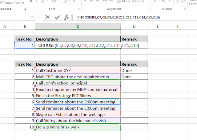
The way CHOOSE works is you specify the position of an item you want to pick and then list our all the items. See below how Sam has used it to solve is problem.

CHOOSE checks for what number is in cell B3 and looks through the orderly list of Description field items, then returns the one that is in the position specified in cell B3. The one above should return "Call Customer XYZ" as that is what is in the position 1 in the Description field items.

And below is a similar formula for the Remark.

Let's specify Task number 4.

Let's specify Task number 8.

Another interesting use of CHOOSE is in a Financial Model to select different projections scenarios.


For an in-depth business relevant training on Excel and Business Data Analysis, you can see the details of our next special training session here.

Using Solver To Find How To Make The Most Of Your Resources

Solver is an amazing tool. It's a decision analysis tool that lets you set your goal and set the conditions to adhere to while searching for the best way to achieve your goal.

Let's see an example I have set up. 

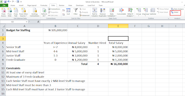
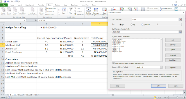
Say we are a new company and have a budget for payroll which we want to maximize to the highest number of staff possible. Below are the details.

So we want Excel to calculate how many Senior Staff, how many Mid-level Staff, how many Junior Staff and how many Fresh Graduate we can employ with the annual budget of N105 million for payroll? And it should take into considerations the following constraints:

• At least one of every staff level
• Maximum of 3 Fresh Graduate
• Each Senior Staff must have exactly 2 Mid-level Staff to manage
• Mid-level Staff must be more than 3
• Each Mid-level Staff must have at least 2 Junior Staff to manage

It's the kind of task you'll use Solver for.

Solver is in Data Menu. 

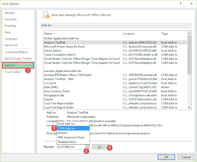
If you don't have it in yours, follow the screenshots below to enable it. Goto Excel Options, Add-ins, Excel Add-ins and enable Solver.

Now you will be able to see under Data menu.

Launch it and set the goal (objective of maximum staff) and the conditions to adhere to.

See the screenshots below for how-to.

And that's all! See the result below.

Congrats! You just did what is referred to as linear programming. You can try include more conditions or use if for your business decision analysis.

How To Enable The Power BI Add-Ins in Excel 2013 and Excel 2016

As long as you have the Office Pro Plus, you can access the Power BI tools. So next is to show you how to find out whether you've got the 2013 or the 2016 version.

How to know which version of Excel you are using

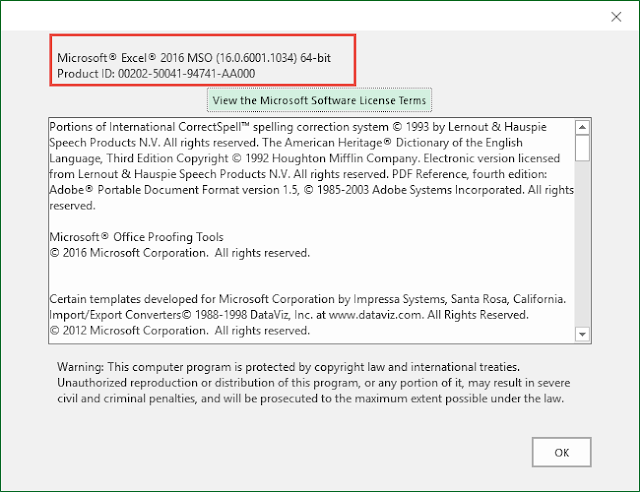
In Excel, go to file and select Account.  Then on the right side of the pane that shows up, click on About Excel.

If you use the 2013 version you will see Excel 2013

If you use Excel 2016, you will see Excel 2016.

For Excel 2013 version

The Power BI add-ins are:

1.       Power Pivot

2.       Power Query

3.       Power Map

4.       Power View

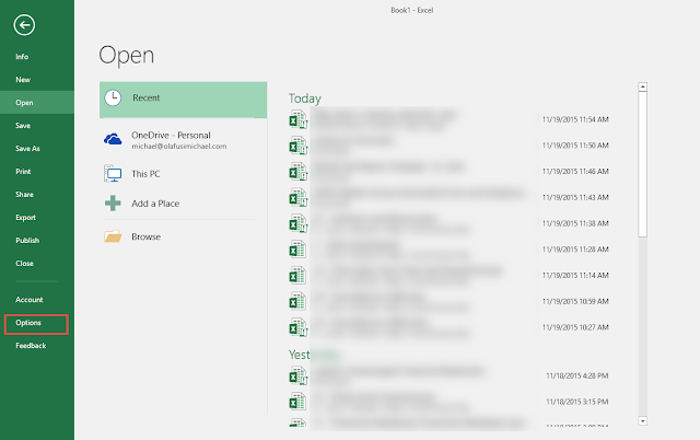
Click on File and Options

In the Window that comes up, click on Add-Ins at the left pane, and select COM Add-Ins.

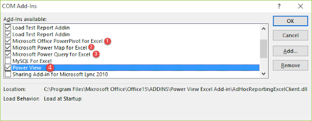
Make sure the four Power BI add-ins are ticked. Then click on OK

.

That will enable/activate the Power BI add-ins.

You will see PowerQuery and PowerPivot on the Menu bar.

You will see the Power Map and Power View under the INSERT menu.

And that’s it for O365 Pro Plus 2013 version.

For Excel 2016 version

For 2016 version, PowerQuery is now an in-built tool (no longer an add-in) and referred to as Get & Transform. Accessible from under Data menu.

For the other three Power BI tools, the activation process is as follows:

Goto File and Options

In the Options Window, click on Add-Ins on the left and select COM Add-Ins.

Tick the PowerPivot, Power Map and Power View add-ins.

PowerPivot shows up on the Menu bar

Power Map is under Insert menu. It has a new name – 3D Maps.

Power View, is a little tricky to access in Excel 2016.

You have to go through the following steps to make it active.

Go to file and click on Options.

In the Options window click on Customize Ribbon.  In the left pane, choose All Commands. Then scroll down to Power View and add it to your Ribbon.

And that’s it.